I Studied Millions of Portfolios. Here's What Actually Kills Compounding

The cost that never shows up on your statement is the one doing the most damage.

Opportunity cost is one of the most destructive forces in investing. It is also one of the most overlooked.

The wealth it destroys never shows up on a statement, which makes it hard to see, hard to study, and easy to ignore.

So I simulated millions of portfolios to pin down where opportunity cost starts, what amplifies it, and how to reduce it in practice.

Here’s what the data shows.

The Setup

To make the results interpretable, you need the setup.

I start with the same initial universe of stocks and simulate millions of portfolios across the full sample period (2001-2025).

I then vary only a few things: portfolio size, turnover, sell rules, and what gets bought after a sale.

Everything else stays fixed: same starting list, same return paths, same horizon. Only the decision rules change.

The point is to isolate the cost of cutting compounding trajectories.

Full methodology and limitations are at the end of the post.

Where Does Opportunity Cost Actually Begin

A buy opens exposure to a range of possible futures. A sell closes that exposure.

The moment you sell, an open trajectory is replaced by a fixed outcome. Once sold, that future no longer belongs to us. That is where opportunity cost begins.

In plain terms: Opportunity cost = a better outcome that was available to you − the outcome you realized.

So the main driver isn’t buying. It’s selling.

The catch is that selling’s damage doesn’t show up immediately. It shows up over time, so we need to track how opportunity cost evolves.

The chart below shows the evolution of opportunity cost across millions of portfolios over 25 years.

The y-axis is logarithmic. On a log scale, a linear trend reflects exponential growth.

Oracle replacement rule (see full methodology). Chart by the author.

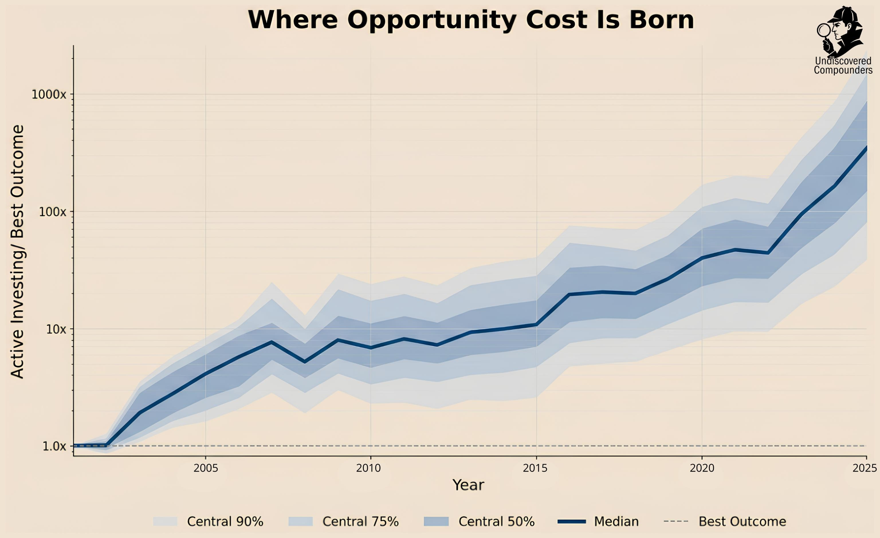
So, opportunity cost doesn’t just add up. It compounds.

And the sudden step-ups make the mechanism visible: those jumps often come from selling positions that later turned into outsized winners.

Fortunately for us, not all sales are created equal.

Why Does It Become So Destructive?

This is where things get interesting.

I simulated three types of selling behavior:

• Selling psychological losers → positions whose current price is below their average purchase price

• Selling at random

• Selling psychological winners → positions whose current price is above their average purchase price

Which type of selling creates the most opportunity cost?

Take a few seconds to think about it.

Beyond the potential mind-blowing effect, active engagement increases the ROI of your reading time.

Here is the result:

Chart by the author.

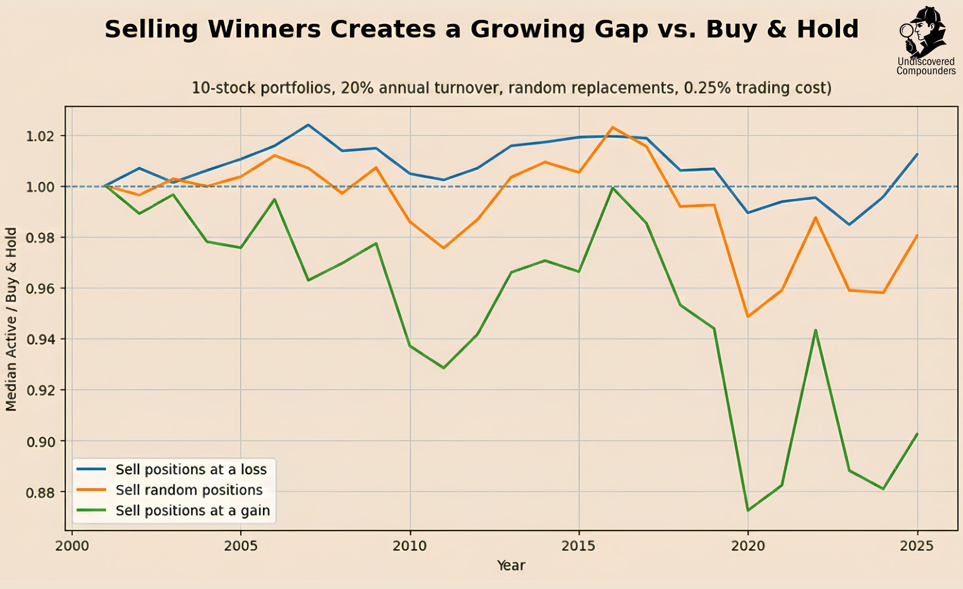
This is the first major finding of the simulation:

• Selling psychological losers leads to lower opportunity cost than buy-and-hold.

• Buy-and-hold leads to lower opportunity cost than selling psychological winners

Even better, in terms of performance: selling psychological losers > selling random > selling psychological winners.

In practice, great compounders tend to be found among stocks that have already gone up, not among those that have gone down.

On average, selling winners gives you a slightly higher chance of cutting off a trajectory that still had exceptional upside ahead.

That asymmetry may look small in the short run. Over long periods, it becomes brutally destructive.

This is Peter Lynch’s “selling your winners and holding your losers is like cutting the flowers and watering the weeds,” but shown here in a more systematic way.

The value of the simulation is that it ignores the subjective “reasons” investors cite for selling and focuses only on the decision rule. Across millions of portfolios, that framework already covers a huge variety of paths and outcomes.

But the mean result is only part of the story. The distribution of selling costs matters just as much:

Chart by the author.

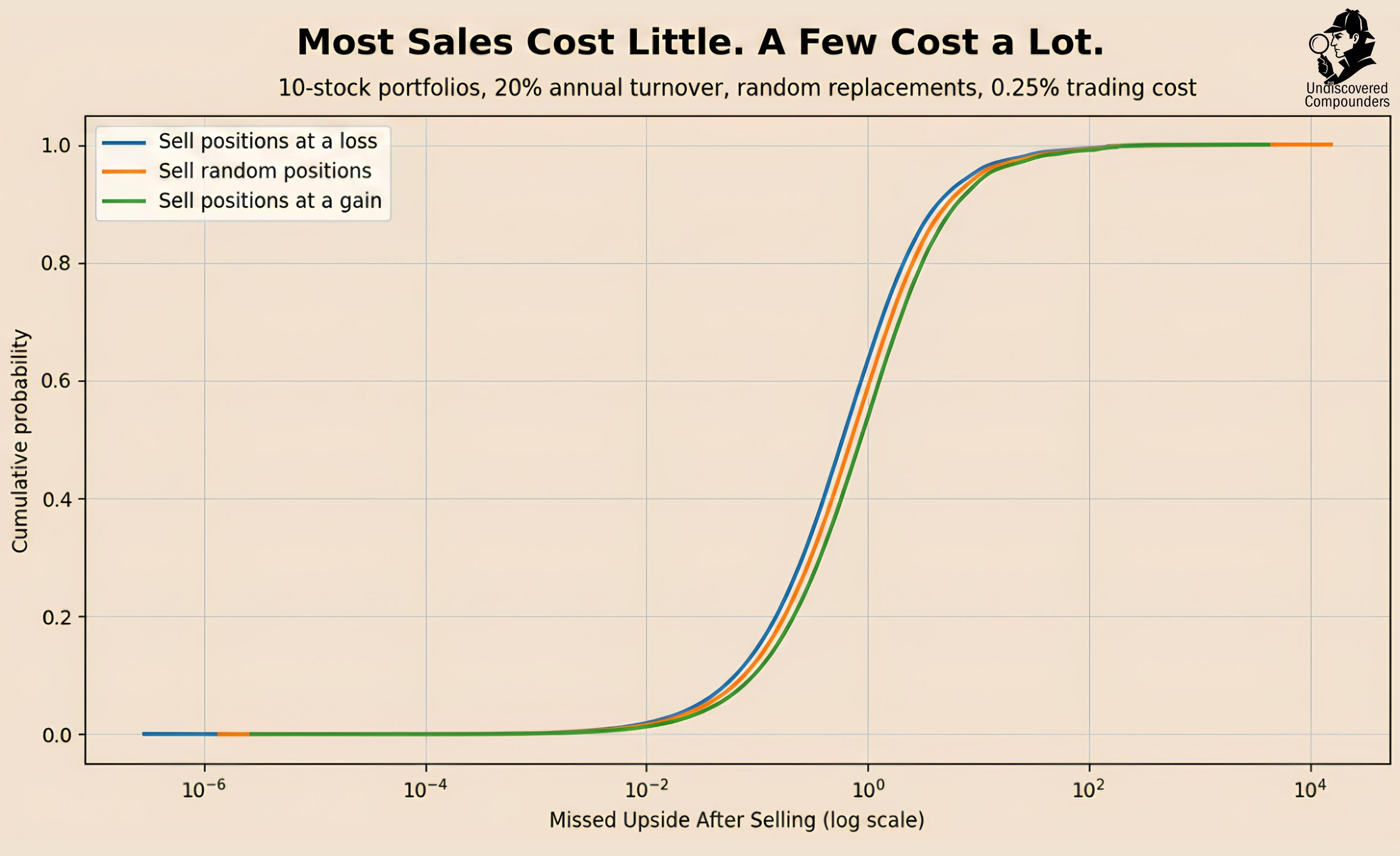
Visually, the differences look subtle. The consequences aren’t.

• This chart shows that most sales impose only a small opportunity cost. The curves rise steeply at low levels, which means a large share of sales do relatively little damage

• But a small minority of sales are catastrophically expensive. Those extreme mistakes happen far less often when selling psychological losers than when selling psychological winners (the green and yellow curves are shifted to the right).

That is the real mechanism.

The destructiveness of selling does not come from every sale being costly. It comes from the fact that a few sales are catastrophic, and selling winners increases both the frequency and the magnitude of those catastrophic errors.

A useful analogy is Russian roulette.

In investing, opportunity cost works like a game in which:

• you do not know how many chambers are in the cylinder,

• you do not know how many bullets are loaded,

• and each sale is a pull of the trigger.

Selling winners is like adding more bullets to the cylinder, and making them larger. The bad outcomes become both more frequent and more severe. Selling losers does the opposite.

But it can get even worse. In fact, it often does. And this time, you are the culprit.

What Amplifies It?

We’ve identified the direct trigger: selling a great compounder. But two factors make that mistake more likely, and more expensive.

1) Portfolio size

A larger portfolio doesn’t just “diversify.” It increases the odds you’re holding a true compounder.

And opportunity cost doesn’t come from owning a compounder. It comes from selling one.

So I hold the number of sales constant and increase portfolio size.

Chart by the author.

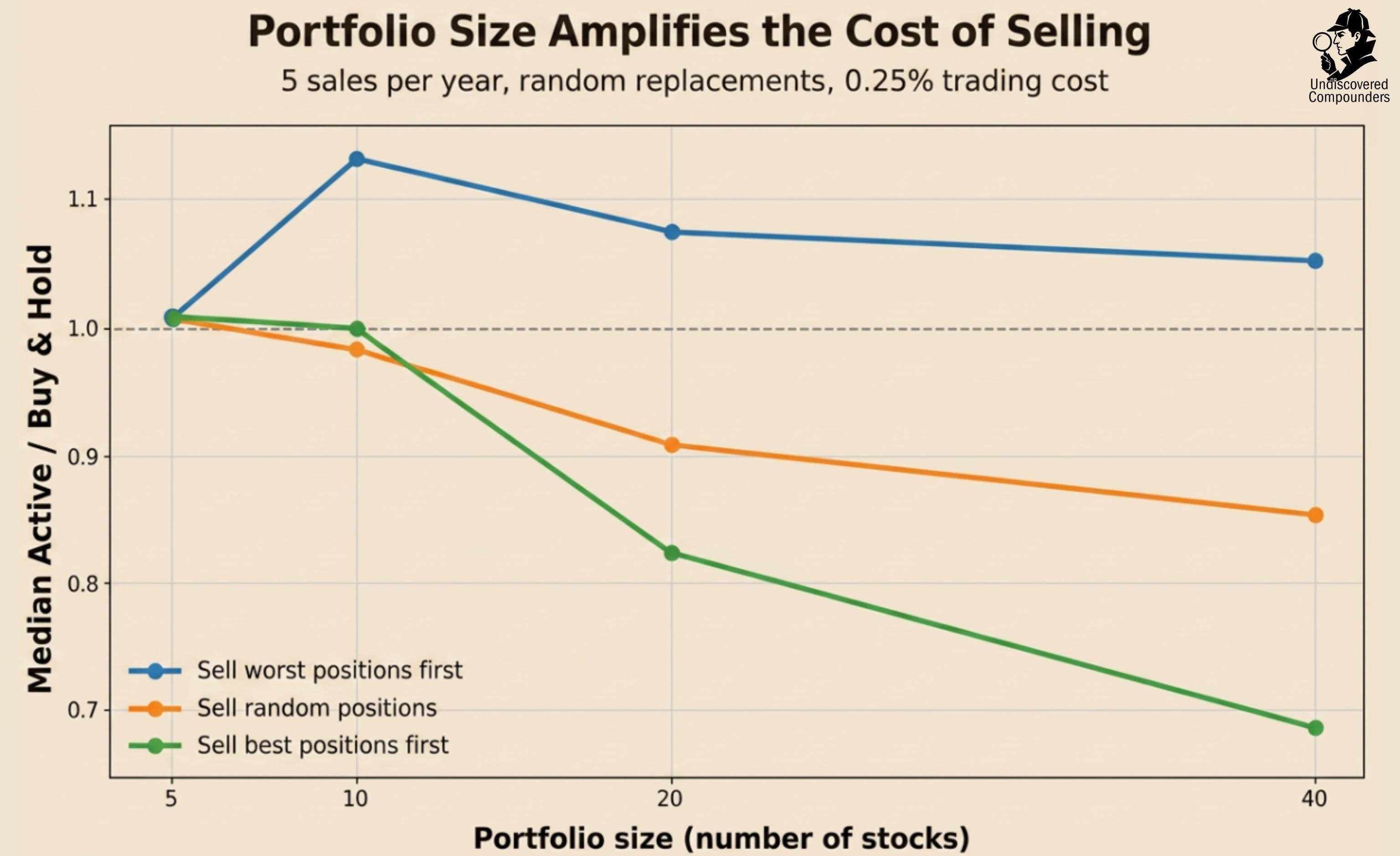
The pattern is clean: as portfolio size grows, opportunity cost grows. Even without trading costs. Even by selling randomly.

Why? Because more names means more chances to own a rare winner, and then “accidentally” cut it.

That’s also why selling psychological winners gets more destructive as portfolios get larger: the “top performer” in a 40-stock portfolio is simply more likely to be a real compounder than the top performer in a 10-stock portfolio.

One detail matters: the small “step up” for sell-worst from 5 → 10 stocks isn’t magic. With 5 sales/year, a 5-stock portfolio is basically full churn, so even “sell-worst” quickly forces you to sell winners. At 10 stocks, you can sell 5 names while still leaving the top winners untouched, temporarily at least.

But the headline doesn’t change: bigger portfolios amplify the cost of selling.

2) Selling frequency (for a fixed portfolio size)

Which brings us to the second amplifier: turnover.

This is the most striking chart in the analysis.

Each curve says a lot, so let’s analyze them one by one.

Chart by the author.

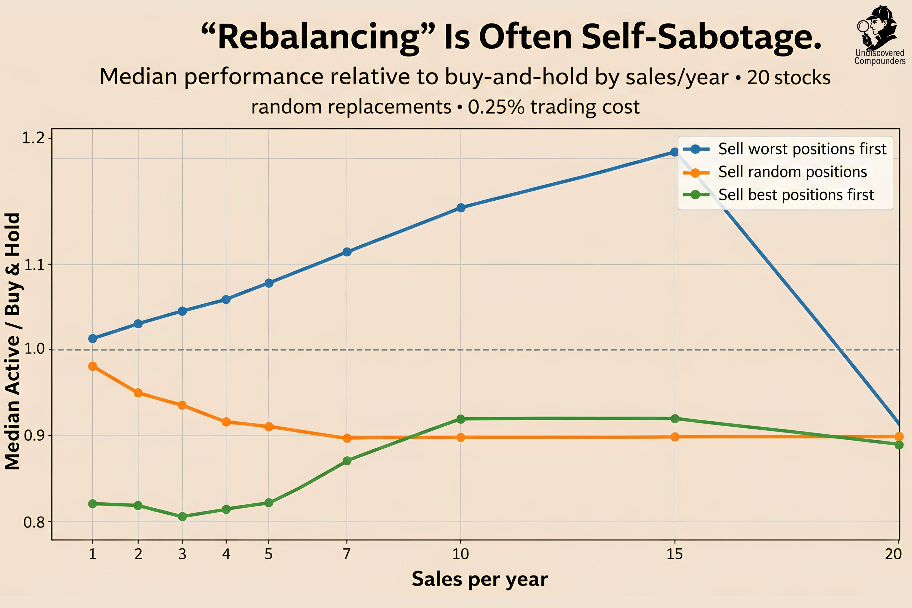
Sell random positions

Start with the simplest case.

Each additional sale pushes performance further below buy-and-hold. In other words, each sale adds opportunity cost.

And that cost is not just financial. Every sale also consumes time, attention, and conviction, only to leave you worse off than if you had done nothing.

In the Russian roulette analogy, higher turnover means pulling the trigger more often.

At first, the damage rises quickly. Then it begins to flatten around 35% turnover (7 sales per year in a 20-stock portfolio).

The reason is simple: at high enough turnover, two opposing effects begin to offset each other. More selling creates more chances to cut off future compounders, but it also creates more chances to buy new ones. What emerges is a negative statistical equilibrium: still worse than buy-and-hold, but no longer deteriorating at the same rate.

The sell-best and sell-worst rules are, in a sense, mirror images of each other.

Sell the best position

This rule is brutally expensive from the start. Your top performer is one of the most likely places to find a stock with exceptional upside still ahead.

As turnover rises, the damage increases. But not forever. In a 20-stock portfolio, once you sell enough names, the “best remaining position” eventually becomes the worst loser.

Sell the worst position

The logic is reversed.

At low turnover, selling the worst position helps because you remove the weakest names first. As turnover rises, that benefit grows, for a while.

But here too, there is a limit. Once enough losers have been sold, the “worst remaining position” eventually becomes the best winner.

That is why the curves start far apart, then move closer together as turnover approaches 100%.

At that point, the sell rule matters less, because the same stocks are increasingly being sold under different labels. Replace the whole portfolio every year, and “sell the best,” “sell the worst,” and “sell random” all converge toward roughly the same outcome: persistent underperformance versus buy-and-hold.

Let’s note something important: performance typically improved when sales came from the bottom 75% of the portfolio. That fact, surprising as it is, will matter later.

---

The conclusion is simple: portfolio size and turnover both amplify opportunity cost.

Each additional sell is another chance to cut off a compounding trajectory.
Each additional stock is another chance to own one, and eventually sell it.

In the end, the biggest driver is what you do with your biggest winners.
And the more stocks you own, the more that decision matters.

How to Reduce It in Practice?

Let’s summarize the key findings:

• Opportunity cost is created at the moment of selling. Reallocation has limited power to offset it.

• In both performance and opportunity cost: sell psychological losers > sell random > sell psychological winners.

• The higher the turnover and the larger the portfolio, the higher opportunity cost tends to be.

• Selling winners is even more destructive in larger portfolios.

These results imply a few practical rules to minimize opportunity cost and maximize long-term performance.

I’m ranking them from least important to most important.

5) The Reallocation Trap

In a reallocation, the opportunity cost from the sale is often larger than the expected benefit from the new buy (when it isn’t a loss).

You can make a “smart” purchase and still make a terrible decision, if you funded it by selling the wrong stock.

Prioritize your reasons to sell, not your reasons to buy.

4) Reduce Portfolio Size

A well-built portfolio of 10 stocks can already capture most diversification benefits without sacrificing performance.

Beyond 15 names, you often drift into “diworsification”: diluted conviction and performance disguised as prudence.

More stocks doesn’t mean less risk. It means more ways to make the one mistake that matters.

3) Build a System That Limits Turnover

Most lifetime performance comes from a few extreme winners.

Those stocks are rare. And they require time.

Every additional sale is another chance to cut a compounding trajectory before it does its job.

Reduce the number of sell decisions. Period.

2) Sell Your Losers Ruthlessly

In the simulation, losers were sold each year and defined in the simplest way possible: the stock trading furthest below its average cost.

Crude rule. Powerful effect.

Why? Because you’re far less likely to find a future great compounder among your current losers, and more likely to find one in what replaces them.

And remember: performance improved almost every time a sale came from the bottom 75% of the portfolio. “Loser” is a wide category here. In practice, it basically means: anything that isn’t one of your true winners.

Sell your losers. Let your capital search for better futures.

1) Protect Your Biggest Winners

If you only remember one thing, make it this:

Selling your winners, those farthest above your cost basis, should be exceptional. Maybe even never, as a routine.

Losses are capped at -100%. Gains have no ceiling.

One true compounder can pay for a lifetime of losers, including stocks that looked like winners at some point and then weren’t.

The most telling result in the analysis was brutally simple: the best setup by far was effectively selling everything each year except the top 5 performers.

Not a magic rule, but a clear message.

You don’t get rich taking profits. You get rich by not touching the winners.

Take care,

Masters of Compounding

Disclaimer: I am not a licensed financial advisor, and nothing in this post should be interpreted as financial, investment, legal, or tax advice. The views expressed here are my own and are provided for informational and educational purposes only. Any investment involves risk, including the risk of loss of capital. You should do your own due diligence and consult a qualified professional before making financial decisions.

Full Methodology and Biases

This analysis uses a deliberately simplified simulation framework designed to isolate one thing: the opportunity cost created by selling.

The simulation starts from a fixed initial cohort of stocks. The cohort includes every stock with a valid year-end price at the end of 2000, and all portfolios are formed from that same starting universe. No late entrants are added later. The sample then runs from 2001 through 2025 using annual data only, with each year represented by the last available price of that year.

Each simulated portfolio is equal-weighted at inception. Portfolio sizes vary across scenarios, and millions of portfolios are randomly drawn for each configuration. A portfolio is then evolved over the full sample period under a specified decision rule. The key variables changed across simulations are portfolio size, turnover, the sell rule, and the buy rule. Everything else is held constant: same starting universe, same return paths, same horizon.

The purpose of this structure is not to mimic real life perfectly. It is to make the effect of selling decisions measurable.

Portfolio evolution

At the end of each year, portfolio positions are repriced using the year-end price of each stock. If a stock later disappears from the dataset, its value is frozen from that point onward rather than forcing a delisting assumption or a terminal loss. This avoids injecting a separate modeling choice into the results. When replacement is impossible, cash is used as a fallback.

All rebalancing takes place only within the initial cohort. In other words, the simulation does not reopen the universe each year and does not allow the purchase of stocks that were not already in the starting set. This is intentional: it keeps the analysis focused on the cost of cutting existing trajectories rather than on the benefits of discovering new names.

Sell rules

Three sell rules are used:

• Random selling: positions are sold at random.

• Psychological winner selling: positions with the largest unrealized gains relative to average purchase price are sold first.

• Psychological loser selling: positions with the largest unrealized losses relative to average purchase price are sold first.

When multiple positions are sold in the same year, the rules are applied in order. Under winner selling, the biggest winner is sold first, then the second biggest, and so on. Under loser selling, the biggest loser is sold first, then the second biggest, and so on.

The core intuition is behavioral rather than fundamental. The simulation is not trying to determine whether a sale was justified by valuation, business quality, or thesis deterioration. It is asking a narrower question: what happens when the decision process is systematically tilted toward selling the strongest winners, the weakest losers, or selling without bias?

Buy rules

Two replacement rules are used:

• Random replacement: replacement positions are chosen randomly from the eligible names not already held.

• Oracle replacement: replacement positions are chosen ex post from the same eligible universe based on their future terminal performance.

The oracle rule is not meant to be realistic. It is a stress test. It asks whether even the best possible replacement, with hindsight, can fully offset the cost created by the sale. In most cases, it cannot.

Benchmarks and definitions

The primary benchmark is buy-and-hold. For each simulated portfolio, the corresponding buy-and-hold benchmark is the portfolio that keeps the same initial positions over the same period, with no turnover. This makes the comparison internally coherent: same starting cohort, same names, same horizon, different decision process.

Opportunity cost is measured in two related ways.

First, at the portfolio level, it is the gap between the realized outcome of the active selling process and the outcome of the benchmark or comparison path.

Second, at the event level, it can be framed as the difference between what a sold position would have become if kept and what the replacement position actually became after transaction costs.

These are different views of the same mechanism: selling closes one path and forces capital onto another.

Why annual data

The simulation uses annual observations rather than daily or monthly data. This reduces noise, keeps the experiment interpretable, and focuses attention on the long-run compounding consequences of selling rather than on short-term fluctuations. That also means the analysis is about structural opportunity cost, not execution timing.

Main biases and limitations

This framework is intentionally narrow, and that creates several biases.

1. Fixed initial cohort bias.
The investable universe is frozen at the starting date. Real investors can discover new companies over time. This setup excludes that possibility. It therefore isolates the cost of abandoning existing winners, but it likely understates the value of skill in finding new names later.

2. Annual frequency bias.
All decisions happen once per year using year-end prices. Real selling decisions are continuous, not annual. This means the simulation captures broad directional effects, not the exact path that would occur under real trading behavior.

3. No thesis-level information.
The model does not know whether a company deteriorated fundamentally, became obviously overvalued, cut guidance, or faced permanent impairment. It only sees prices and rules. So the results should not be read as “never sell.” They should be read as evidence that selling is far more expensive than it appears by default.

4. No taxes, slippage, or market impact beyond simple trading costs.
Transaction costs are modeled mechanically, but taxes and execution frictions are not. In real life, those frictions usually make selling look even worse.

5. Equal-weight simplification.
All portfolios start equal-weighted. That makes cross-scenario comparisons cleaner, but it is not how all real portfolios are run. Capital allocation skill is not modeled here.

6. Survival and disappearance handling.
When a stock stops having prices in the dataset, its value is frozen rather than treated as a realized delisting return. That is a conservative modeling choice for consistency, but it is still a choice. Different assumptions would slightly change the tails.

7. Psychological winner/loser definitions are price-based, not fundamental.
A “winner” is defined as a position with an unrealized gain relative to average purchase price, and a “loser” as a position with an unrealized loss. The sell rules rank positions by that price-based measure, not by fundamentals or intrinsic value. A stock can be above cost and still cheap, or below cost and still bad.

8. Opportunity cost is partly path-dependent.
The exact magnitude of opportunity cost depends on which future extreme winners were owned, when they were sold, and what replaced them. That means the results should be interpreted statistically, not as deterministic laws for every individual case.

What this framework is good for

This simulation is useful for answering general questions about the consequences of selling, not for judging specific real-world decisions.

It is not meant to determine whether any single sale was justified. Its purpose is to show that, as a class of actions, selling is far more dangerous than most investors assume.

That is the main point.